Background
Having a good pre-trained language model can be significant time and money saver (better results for less compute and time) for NLP projects. Empirical studies have shown that unsupervised pre-training greatly improves generalization and training in many machine learning tasks. For example according to
this paper from Montreal and Google:
The results suggest that unsupervised pretraining guides the learning towards basins of attraction of minima that support better generalization from the training data set;
Thankfully, almighty Google scientists made some of their models open and available for everyone to use. Here, we will utilize Google's
lm_1b pre-trained TensorFlow language model. Vocabulary size of the model is 793471, and it was trained of 32 GPUs for five days. If you want to learn the details, please refer to
this paper. The entire TensorFlow graph is defined in a protobuf file. That model definition also specifies which compute devices are to be used, and it set to use primary CPU device. That's fine, most of us will not be able to fit the large model parameters into conventional desktop GPU anyway.
The original
lm_1b repository describes steps somewhat awkwardly. You need to do some manual work, and run Bazel commands with arguments to use the model. If you want get embeddings, you need to again run Bazel commands with your text in the parameters and it will save results into a file. On top of that, their inference and evaluation code is written for Python 2. The code and instructions provided here allow you to fetch embeddings in a run-time of a Python 3 code in more flexible manner.
Setting Up
Before you start, make sure you are working on a modern system with at least 20 Gb of RAM. In its raw form, Google's model has 1.04 Billion parameters. My relatively powerful system has 16 Gb of RAM, and with couple of open Chrome tabs, the model is unable to fit the parameters into the memory. Therefore, the work was done on a Google Cloud instance with 26 Gb of RAM.
Download the weights, checkpoint, and the graph definition
Let's say that you are working in a project folder called 'my_project'. To fetch the pre-trained model, execute bash code provided below. You can either
download the code and run it, or just copy and paste this into your terminal. Note that entire model weighs around 4 Gb, so it might take some time for the script to finish executing.
Inference
We have our pre-trained model ready. Now, we will write a Python module that will help our projects to interface with the model. First, we need to import some libraries and declare a function that will load the model graph from protobuf definition:
Next, we initialize our variables and tensors.
Now, we can define a function that can compute embeddings. This specific function below propagates through entire text it's given.
This brings us to the conclusion. You can pass some text to the
forward function and get embedding for the entire text, which is final state of the recurrent network after propagating through the provided text. Below, you can find example of applying the model to text from
USA.gov and
Cosmopolitan.com. Some of the text samples acquired from USA.gov:
"Privately owned, subsidized housing in which landlords are subsidized to offer reduced rents to low-income tenants"
"Each state or city may have different eligibility requirements for housing programs. Contact your local Public Housing Agency to learn about your eligibility for Housing Choice Vouchers"
"The Eldercare Locator is a free service that can connect you with resources and programs designed to help seniors in your area"
Here are the example text sampled from Cosmopolitan.com.
"A shocking number of women have trouble mentally letting go and enjoying oral sex when their partner goes down on them"
"While very few things are going to recreate the feeling of a tongue exactly, some newer vibrators come pretty close"
"Neither one of you can read each other's mind during sex, so speak up if there's something that you want that he's not delivering"
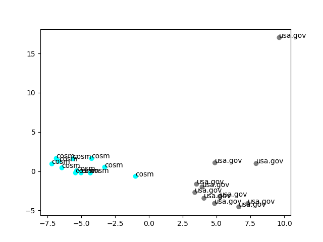
Results are very good. As you can see in the plot below, texts from the same sources cluster together. Since the original embedding are 1024 dimensional and we are simply projecting them with PCA for visualization, representation is not perfect, thus we see a point far away from the rest.
Full source code can be found
here.
Thank for reading! Hope you will have fast convergence and small losses on your test sets.