Introduction
Batch Normalization is a simple yet extremely effective technique that makes learning with neural networks faster and more stable. Despite the common adoption, theoretical justification of BatchNorm has been vague and shaky. The belief propagating through the ML community is that BatchNorm improves optimization by reducing internal covariate shift (ICS). As we shall see, ICS has little to no effect on optimization. This blog post looks at the explanations of why BatchNorm works, mainly agreeing with the conclusions from: How Does Batch Normalization Help Optimization? (No, It Is Not About Internal Covariate Shift) [1]. This works joins the effort of making reproducibility and open-source a commonplace in ML by reproducing the results from [1] live in your browser (thanks to TensorFlow.js ). To see the results you will have to train the models from scratch, made as easy as clicking a button. Initialization of parameters is random, therefore you will see completely different results every time you train the models. Source code to the models presented here can be found in this GitHub repo.
Batch Normalization, Mechanics
Batch Normalization is applied during training on hidden layers. It is similar to the features scaling applied to the input data, but we do not divide by the range. The idea is too keep track of the outputs of layer activations along each dimension and then subtract the accumulated mean and divide by standard deviation for each batch. Interactive visualization below explains the process better.
Step 1: Subtract the mean
Calculate batch mean: `\mu_\B ← 1/m Σ(x_i)`
Subtract the mean: `\hat{x}_i ← x_i - \mu_B`
Subtracting the mean will center the data around zero. Click the button to demonstrate the effect.
Make sure to randomize the data if you want to subtract the mean again. Pay attention to the axes.
Step 2: Normalize the Variance
Calculate Variance: `\sigma_B^2 ← 1/m Σ((x_i - \mu_B)^2)`
Subtract the mean, divide by standard deviation: `\hat{x}_i ← (x_i - \mu_B) / \sqrt(\sigma_B^2 + \epsilon)`
Subtracting the mean and dividing by the square root of variance, which is basically standard deviation, will normalize the data variance. Here, `\epsilon` is a negligibly small number added to avoid division by zero. Click the button, pay attention to the axes.
Important thing to note is that traditionally, Batch Normalization has learnable parameters. After the steps shown above we learn linear transformation: `y_i ← γ * \hat{x_i} + β` where `γ, β` are the learned parameters and `y_i` is the output resulting from the BatchNorm layer. So in case BatchNorm is actually not needed, these parameters will learn the identity function to undo the Batch Normalization. BatchNorm behaves differently during test time. We no longer calculate the mean and variances but instead use what we have accumulated during training time by using exponential moving average.
Does Batch Normalization Work?
Before we look at the plausible reasons of why BatchNorm works let's convince ourselves that it actually works as well as it's believed to. We will train a CNN with and without BatchNorm, on low and high learning rates. The default CNN architectures we will be using are shown below. To the left is the regular convolutional neural network and to the right is the same network with addition of batch normalization after each convolution.
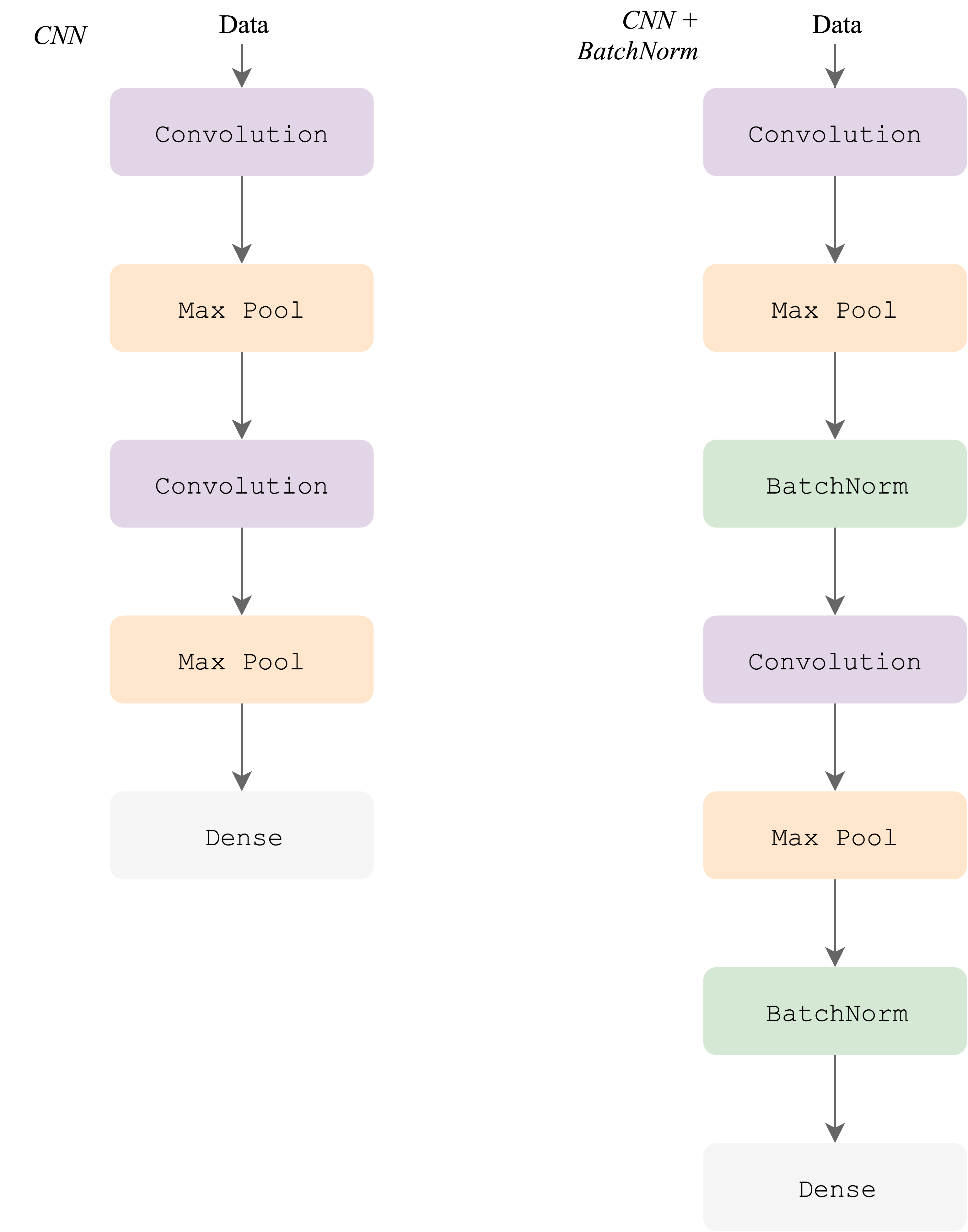
Architecture used in this post
We are going to train digit classifier using the good ol' MNIST dataset. Below, you can train these two models right in your browser, just click Train. After you start training, please give it minute or less to finish training, otherwise the page might lag.
Evaluation of the CNN vs CNN with BatchNorm on the test set during training with different learning rates.
Now the training is complete, hopefully you see that with both learning rates, BatchNorm performs better. It's not unusual for the standard CNN without BatchNorm to get lost and diverge with higher learning rate, where with BatchNorm it just trains faster.
Internal Covariate Shift
According to the original BatchNorm paper [3], the trick works because it remedies the Internal Covariate Shift (ICS). ICS refers to the change of distribution of inputs to the hidden layers as the parameters of the model change. Concretely, shift of the mean, variance, and change in distribution shape. Intuitively this explanation feels correct. Let's say in the beginning, activations of the first layer look gaussian centered at some point, but as training progresses, entire distribution moves to another mean and becomes skewed, potentially this confuses the second layer and it takes longer for it to adapt. But as [1] shows, this reasoning might not be correct. Their results show that ICS has little to do with optimization performance, and BatchNorm does not have significant effect on ICS.
Error Surface
Even before BatchNorm was mainstream, Geoffrey Hinton showed how shifting and scaling the inputs can reshape the error surface. As he explained in his Neural Networks Course (Lecture 6.2 — A bag of tricks for mini batch gradient descent), centering data around zero and scaling gives each dimension similar curvature and makes the error surface more spherical as oppose to high curvature ellipse.
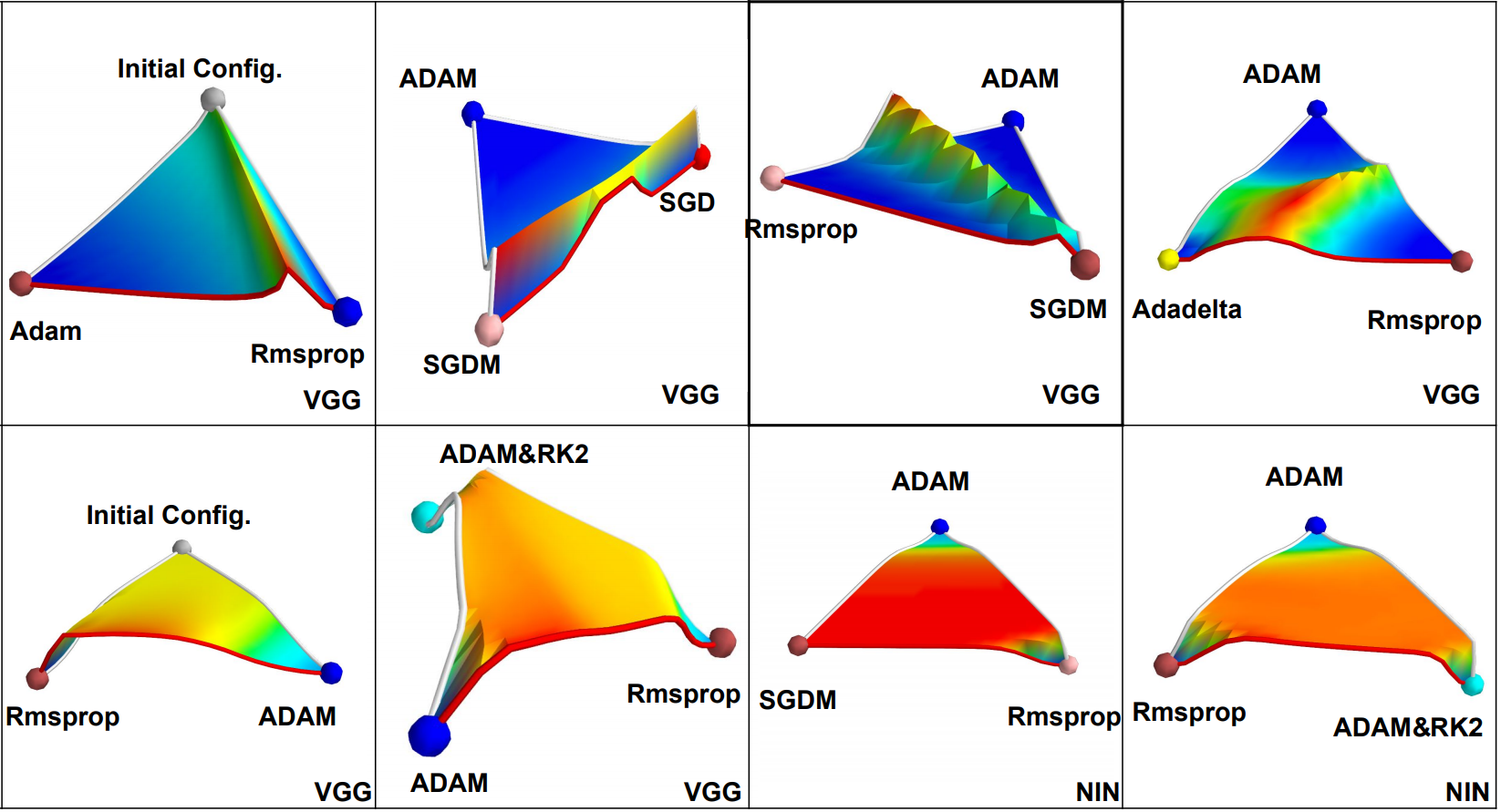
Visualization of the Loss Surface with (top) and without (bottom) batch-normalization. Source: [2]
Empirical work done by D. Jiwoong et al. [2] (figure above) observed sharp unimodal jumps in performance with batch normalization, but without batch normalization they reported wide bumpy shapes that are not necessarily unimodal. They also discovered that without BatchNorm, optimization performance depends highly on the weight initialization. Their research suggests that BatchNorm makes network much less dependent on the initial state.
Fundamental Analysis
Authors of [1] offer their fundamental analysis of BatchNorm's effect on optimization. They provide both empirical evidence and theoretical proof that BatchNorm helps optimization by making optimization landscape smoother rather than reducing ICS. As we shall see, results suggest ICS might even have no role in optimization process. They formalize their argument by showing that BatchNorm improves Lipschitzness of both the loss and the gradients. Function `f` is known to be `L`-Lipschitz if `||f(x_1)-f(x_2)|| <= L||x_1-x_2||`. Lipschitzness of the gradient is defined by `β`-smoothness, and `f` is `β`-smooth if the function gradients are `β`-Lipschitz: `||∇ f(x_1)- ∇ f(x_2)|| <= β ||x_1-x_2||` where `x_1` and `x_2` are inputs. They as well show that batch norm is not the only way of normalizing the activations to smoothen the loss landscape. They show that their `l_1`, `l_2`,l_{max} normalization methods provide similar benefits, although they can introduce higher ICS. To see these normalization results and the mathematical proofs please refer to the paper. I personally believe this type of fundamental research is very important not only for understanding but also for cultivating ML research culture which builds on first principles.
We are now going to see that BatchNorm has no significant effect on ICS, and that ICS neither hurts or improves optimization. We will be training three different models: Regular CNN, CNN with BatchNorm, and CNN with BatchNorm injected with noise (right after BatchNorm). The noise sampled from a non-zero mean and non-unit variance distribution, and such noise introduces chaotic covariate shifts, yet the model still performs better than regular CNN. When ready, go ahead and smash dat train button.
Evaluation of the models on train set (top) and change of activation moments (mean & variance) between successive steps (bottom)
After training you should see that BatchNorm with or without noise performs better than regular CNN. Also, in the bottom two charts you should see in case of the BatchNorm with noise, moments (mean & variance) of the activations fluctuate like crazy. So we are intentionally introducing ICS, yet the model still performs better. This supports the argument put forward by the authors.
We are going to train CNN vs CNN + Batch Norm for the last time to look at the smoothness effect that BatchNorm introduces. Left chart shows how loss changes between each training step, and the right chart shows "effective" `β` smoothness observed while interpolating in the direction of the gradient. The "effective" `β` refers to the fact that we can't achieve global `β` smoothness due to the non-linearities, but we can approximate local "effective" `β` smoothness. Lower and less fluctuating values indicate smoothness.
Loss change between successive steps (left) and "effective" `β`-smoothness (right)
The local `β`-smoothness above is computed as follows: we pick some range `a`, and every training step `t` we travel in that range and calculate `max_a || ∇ f(x_t) - ∇ f(x_t - a * ∇ f(x_t)) || / || a * ∇ f(x_t) ||` where `∇ f` is the gradient of the loss with respect to `x_t` - activation of convolution/BatchNorm layer.
References
1. How Does Batch Normalization Help Optimization? (No, It Is Not About Internal Covariate Shift); Tsipras, Santurkar, et. al.; https://arxiv.org/pdf/1805.11604.pdf; (5 Jun, 2018)2. An Empirical Analysis of Deep Network Loss Surfaces; Daniel Jiwoong, Michael Tao & Kristin Branson; https://arxiv.org/pdf/1612.04010v1.pdf; (13 Jun, 2016)
3. Batch Normalization: Accelerating Deep Network Training by Reducing Internal Covariate Shift; Sergey Ioffe, Christian Szegedy; https://arxiv.org/pdf/1502.03167.pdf; (2 Mar, 2015)